
SK CREATION

SK Enterprise RAG Pipeline

Queries/min
0
+12% vs last hour
P95 Latency
0s
-8% vs last hour
Grounding
0%
+0.4% vs last hour
Cache Hit
0%
+5% vs last hour

Pipeline Stages

Query Understanding Engine

stage 3 / 10

Classifies intent, detects language, rewrites ambiguous queries, and routes to the appropriate retrieval strategy. Handles multi-turn context injection and sensitive query flagging.

Intent ClassificationQuery RewritingPII DetectionRouting

Stage Config

Intent Classes24 enterprise types
Rewrite ModelGPT-4o-mini
Accuracy94.2% intent F1
Latency~180ms
Configuration / Code
class QueryUnderstanding:
    async def process(self, query: str, history: list):
        intent = await self.classifier.predict(query)
        rewritten = await self.rewriter.rewrite(
            query, history, intent
        )
        strategy = self.router.decide({
            "intent": intent,
            "has_filters": detect_filters(query),
            "needs_live_data": intent in LIVE_INTENTS
        })
        return QueryPlan(rewritten, intent, strategy)
Live Data / Action Payload
{
  "action": "QUERY_ANALYSIS_COMPLETE",
  "analysis": {
    "original": "What is our Q3 procurement policy?",
    "rewritten": "Acme Corp procurement policy software licenses Q3 2024",
    "intent": "POLICY_LOOKUP",
    "entities": {
      "timeframe": "Q3 2024",
      "department": "Procurement"
    },
    "routing_strategy": "HYBRID_BROAD_SEARCH",
    "pii_detected": false
  }
}
Query Simulator

Platform Services Health

Vector Store
23ms
Elasticsearch
18ms
Azure OpenAI
1.1s
Cohere Rerank
210ms
OPA Policy Engine
4ms
Salesforce CRM
940ms
SAP ERP
380ms
Redis Cache
1ms

Global Pipeline Stats (24h)

Total Queries

12,847

Avg Latency

2.1s

Cache Hits

34.7%

Grounding Pass

98.2%

Rejection Rate

1.8%

Tokens Gen

4.2M

RAG fundamentals

What is RAG and why does it exist?

RAG (Retrieval-Augmented Generation) solves the fundamental limitations of LLMs: they have a fixed knowledge cutoff, cannot access private data, and hallucinate when forced to recall specific facts. The core idea: instead of asking the model to memorize everything, you retrieve relevant documents at query time and inject them as context. The model becomes a reasoning engine over supplied evidence, not a knowledge store.

The two halves of RAG

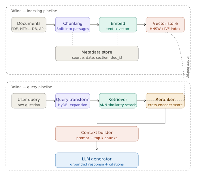
The pipeline splits cleanly into an offline indexing phase (run once, or incrementally) and an online query phase (runs per request). Click any box in the diagram to drill deeper into a component.

RAG pipeline overview — offline indexing and online query phases

Offline indexing (top) · Online query pipeline (bottom) · Dashed line = index lookup

Phase 1 — OfflineStep 1

Document ingestion

Raw sources enter through connectors that parse, normalize, and prepare text for chunking.

You ingest raw sources: PDFs, web pages, SQL tables, markdown docs, APIs. Each source needs a connector that handles parsing (stripping HTML, OCR on scans, handling tables) and normalization into clean text.
Phase 1 — Offline indexing

Phase 2 — Online query pipeline

Retrieval & query strategies

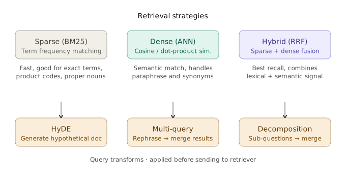
Sparse BM25, dense ANN, and hybrid RRF fusion — plus query transforms (HyDE, multi-query, decomposition) applied before the retriever.

RAG retrieval strategies — sparse BM25, dense ANN, hybrid RRF, and query transforms

Retrieval deep dive

The core insight

Every retrieval method answers: “how do I measure whether this chunk is relevant to this query?” Sparse and dense methods use completely different notions of similarity, which is exactly why they complement each other.

Sparse retrieval (BM25)

Sparse retrieval represents both queries and documents as high-dimensional term-frequency vectors — “sparse” because almost all dimensions are zero (most terms do not appear in any given document). The classic algorithm is BM25 (Best Match 25), which improves on raw TF-IDF by saturating term frequency and normalizing for document length.

BM25 score for document D given query Q

score(D, Q) = Σ IDF(qi) · [f(qi, D) · (k1 + 1)] / [f(qi, D) + k1 · (1 - b + b · |D|/avgdl)]

IDF(qi) = log((N - df + 0.5) / (df + 0.5))

f(qi, D) = term frequency · |D| = document length · avgdl = average doc length · k1 (typically 1.2–2.0) and b (typically 0.75) are tuning parameters

Mechanically: a BM25 index is an inverted index — a map from term → list of (doc_id, score) pairs. Lookup is O(number of query terms × posting list length), which is fast and exact.

Where sparse excels

Exact keyword matching, product codes (iPhone 15 Pro Max), model numbers, proper nouns, technical identifiers — any case where user vocabulary precisely matches document vocabulary. No semantic gap to cross.

Where it fails

Synonyms, paraphrases, and anything requiring conceptual understanding. “Canine dental care” will not retrieve “dog tooth health” with zero overlap.

Dense retrieval (ANN)

Dense retrieval encodes both query and documents as low-dimensional continuous vectors (768–3072 dimensions). Proximity in this space correlates with semantic similarity — “canine dental care” and “dog tooth health” land near each other even with no shared terms.

The architecture is a bi-encoder: pass the query through an encoder to get q_vec, pass each document through the same encoder to get d_vec, and relevance is cosine_similarity(q_vec, d_vec) or dot product. You cannot brute-force compare against millions of vectors per query — this is where ANN (Approximate Nearest Neighbor) indexing comes in.

  • HNSW (Hierarchical Navigable Small World): multi-layer graph with greedy traversal from coarse to fine — like a skip list. ~95–99% recall at ~1–5ms per query. Default for most RAG deployments.
  • IVF (Inverted File): k-means clusters vectors; query probes only nearest clusters. More memory efficient but generally lower recall at the same speed.

Where dense excels

Semantic similarity, paraphrase, cross-lingual retrieval, conceptual questions.

Where it struggles

Rare technical terms, product codes, exact strings — the embedding model may map them to similar-looking but meaningless positions in the space.

Hybrid search and Reciprocal Rank Fusion

BM25 and dense retrieval fail in different, mostly non-overlapping ways — so running both and merging is almost always better than either alone. The naive approach — normalize scores from both retrievers and add them — breaks down because BM25 scores (typically 0–30) and cosine similarity (0–1) are on completely different scales.

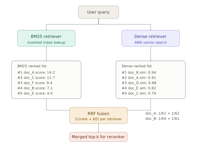
Reciprocal Rank Fusion sidesteps this by ignoring raw scores and working only on rank positions:

RRF_score(doc) = Σ_retrievers [ 1 / (k + rank(doc)) ]

k = 60  (dampens top-rank dominance)

Documents appearing in both lists accumulate scores from both retrievers. Documents in only one list still get credit for that single appearance.

Hybrid search flow — BM25 and dense ANN retrievers run in parallel, ranked lists fused by RRF, merged top-k sent to reranker

Concrete RRF example (from diagram)

  • doc_A: rank 1 in BM25, rank 2 in dense → 1/(60+1) + 1/(60+2) = 0.0325
  • doc_B: rank 4 in BM25, rank 1 in dense → 1/(60+4) + 1/(60+1) = 0.0320

Despite never topping either individual list, doc_A edges out as the hybrid winner. No learned parameters, no normalization — RRF just works, which is why it became the standard.

The decision framework — which to use when

How to reason through the choice in production system design:

When to lean sparse

Your corpus has lots of domain-specific jargon, product codes, model numbers, or acronyms that an embedding model has not seen enough of to position well. Also useful when users are expert searchers who know exactly the terminology in the documents.

When to lean dense

Users ask questions in natural language that may not match document vocabulary. Cross-language retrieval. Conceptual questions ("what is the company's policy on X") rather than keyword lookups.

When to use hybrid

Almost always in production — unless you have a very specific reason not to. Tradeoffs are infrastructure complexity (two indexes) and latency (two parallel requests). Most systems accept this because hybrid consistently beats either approach alone on recall benchmarks.

Practical benchmark: on BEIR, hybrid BM25+dense improves nDCG@10 over dense-only by 2–5 points on most datasets — meaningful but not transformative. Gains are largest on technical corpora (TREC-COVID, SciFact) where terminology matters.

Critical design decisions

Chunk size vs. retrieval granularity

Small chunks retrieve precisely but lose context. Large chunks are self-contained but match queries poorly. Parent-child chunking is the standard production solution: embed small child chunks, retrieve parent chunks for the LLM.

Embedding model selection

Domain-specific models (e.g. medical, legal, code) dramatically outperform general models on in-domain tasks. Always benchmark on your actual data distribution, not MTEB leaderboards alone.

Retrieval metrics

Measure recall@k (does the right chunk appear in top-k?), MRR (how highly is it ranked?), and NDCG. Downstream, measure answer faithfulness (is the answer grounded in context?) and answer relevance (does it address the question?). Tools like RAGAS automate this evaluation.

Failure modes to know

Semantic gap

Query and document do not share vocabulary — dense retrieval misses them.

Context poisoning

A retrieved chunk contains misleading information that steers the answer wrong.

Lost-in-the-middle

Relevant chunk sits in the middle of a long context and the LLM ignores it.

Retrieval-generation mismatch

Retrieved chunks are relevant but the LLM ignores them in favor of parametric knowledge.

Advanced architectures

Agentic RAG adds a routing step where the LLM decides which retrieval strategy to use (or whether to retrieve at all). FLARE and Self-RAG have the model generate in passes, retrieving mid-generation when confidence is low. GraphRAG builds a knowledge graph over the corpus to handle multi-hop reasoning that flat retrieval misses.